 Photo by rawpixel on Unsplash
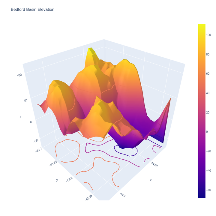
Bedford Bathy Plotting using Python
# Author : Jay Patel
# 3D Bedford basin bathy

import plotly.graph_objects as go

import pandas as pd

# Read data from a csv
z_data = pd.read_csv('bathy_bedford.csv')

fig = go.Figure(data=[go.Surface(z=z_data.values)])

fig.update_layout(title='Bedford Basin Elevation', autosize=True,
                   width=900, height=900,
                   margin=dict(l=65, r=50, b=65, t=90))

fig.show()

# cmap=plt.cm.viridis, linewidth=0.2
fig.update_traces(contours_z=dict(show=True, usecolormap=True,
                                  highlightcolor="limegreen", project_z=True))

Surface Plot With Contours
import plotly.graph_objects as go

import pandas as pd

# Read data from a csv
z_data = pd.read_csv('bathy_bedford.csv')

fig = go.Figure(data=[go.Surface(z=z_data.values)])
fig.update_traces(contours_z=dict(show=True, usecolormap=True,
                                  highlightcolor="limegreen", project_z=True))
fig.update_layout(title='Bedford Basin Elevation', autosize=True,
                   width=900, height=900,
                   margin=dict(l=65, r=50, b=65, t=90))

fig.show()

import plotly.graph_objects as go
import numpy as np
import pandas as pd

# Read data from a csv
z_data = pd.read_csv('bathy_bedford.csv')
z = z_data.values
sh_0, sh_1 = z.shape
x, y = np.linspace(44.66875, 44.74791667, sh_0), np.linspace(-63.69791667, -63.52708333, sh_1)
import plotly.graph_objects as go
import pandas as pd
import numpy as np
# Read data from a csv
z_data = pd.read_csv('bathy_bedford.csv')
z = z_data.values
sh_0, sh_1 = z.shape
x, y = np.linspace(44.66875, 44.74791667, sh_0), np.linspace(-63.69791667, -63.52708333, sh_1)
fig = go.Figure(data=[go.Surface(z=z, x=x, y=y)])
fig.update_traces(contours_z=dict(show=True, usecolormap=True,
                                  highlightcolor="limegreen", project_z=True))
fig.update_layout(title='Bedford Basin Elevation', autosize=True,
                  width=900, height=900,
                  margin=dict(l=65, r=50, b=65, t=90))
fig.update_layout=dict(xaxis=dict(title='Latitude'),
                  yaxis=dict(title='Longitude'))
fig.show()

Configure Surface Contour Levels
import plotly.graph_objects as go
import pandas as pd
import numpy as np

# Read data from a csv
z_data = pd.read_csv('bathy_bedford.csv')
z = z_data.values
sh_0, sh_1 = z.shape
x, y = np.linspace(44.66875, 44.74791667, sh_0), np.linspace(-63.69791667, -63.52708333, sh_1)
# fig = go.Figure(data=[go.Surface(z=z, x=x, y=y)])

fig = go.Figure(go.Surface(
    contours = {
        "x": {"show": True, "start": 44.66875, "end": 44.74791667, "size": 0.04, "color":"white"},
        "z": {"show": True, "start": -63.69791667, "end": -63.52708333, "size": 0.05}
    },
    z=z, x=x, y=y))
fig.update_layout(
        scene = {
            "xaxis": {"nticks": 20},
            "zaxis": {"nticks": 8},
            'camera_eye': {"x": 0, "y": -1, "z": 0.5},
            "aspectratio": {"x": 1, "y": 1, "z": 0.2}
        })
fig.show()

import plotly.graph_objects as go
import pandas as pd
import numpy as np
# Read data from a csv
z_data = pd.read_csv('bathy_bedford.csv')
z = z_data.values
sh_0, sh_1 = z.shape
x, y = np.linspace(44.66875, 44.74791667, sh_0), np.linspace(-63.69791667, -63.52708333, sh_1)
fig = go.Figure(data=[go.Surface(z=z, x=x, y=y)])
fig.update_traces(contours_z=dict(show=True, usecolormap=True,
                                  highlightcolor="limegreen", project_z=True))
fig.update_layout(title='<b>Bedford Basin Elevation</b>',xaxis_title="Latitude",
                  yaxis_title="Longitude",autosize=True,
                  margin=dict(l=65, r=50, b=65, t=90))
fig.update_layout(scene = dict(
                    xaxis_title='Latitude',
                    yaxis_title='Longitude',
                    zaxis_title='Elevation')
                    )
# fig.update_layout(color='Elevation')
fig.update_layout(coloraxis_colorbar=dict(
    title="Elevation",
    thicknessmode="pixels", thickness=50,
    lenmode="pixels", len=200,
    yanchor="top", y=1,
    ticks="outside", ticksuffix="",
    dtick=5
))
fig.show()

import plotly.graph_objects as go
import pandas as pd
import numpy as np
# Read data from a csv
z_data = pd.read_csv('bathy_bedford.csv')
z = z_data.values
sh_0, sh_1 = z.shape
x, y = np.linspace(44.66875, 44.74791667, sh_0), np.linspace(-63.69791667, -63.52708333, sh_1)
fig = go.Figure(data=[go.Surface(z=z, x=x, y=y,colorscale='Viridis')])
"""The 'colorscale' property is a colorscale and may be
    specified as:
      - A list of colors that will be spaced evenly to create the colorscale.
        Many predefined colorscale lists are included in the sequential, diverging,
        and cyclical modules in the plotly.colors package.
      - A list of 2-element lists where the first element is the
        normalized color level value (starting at 0 and ending at 1),
        and the second item is a valid color string.
        (e.g. [[0, 'green'], [0.5, 'red'], [1.0, 'rgb(0, 0, 255)']])
      - One of the following named colorscales:
            ['aggrnyl', 'agsunset', 'algae', 'amp', 'armyrose', 'balance',
             'blackbody', 'bluered', 'blues', 'blugrn', 'bluyl', 'brbg',
             'brwnyl', 'bugn', 'bupu', 'burg', 'burgyl', 'cividis', 'curl',
             'darkmint', 'deep', 'delta', 'dense', 'earth', 'edge', 'electric',
             'emrld', 'fall', 'geyser', 'gnbu', 'gray', 'greens', 'greys',
             'haline', 'hot', 'hsv', 'ice', 'icefire', 'inferno', 'jet',
             'magenta', 'magma', 'matter', 'mint', 'mrybm', 'mygbm', 'oranges',
             'orrd', 'oryel', 'peach', 'phase', 'picnic', 'pinkyl', 'piyg',
             'plasma', 'plotly3', 'portland', 'prgn', 'pubu', 'pubugn', 'puor',
             'purd', 'purp', 'purples', 'purpor', 'rainbow', 'rdbu', 'rdgy',
             'rdpu', 'rdylbu', 'rdylgn', 'redor', 'reds', 'solar', 'spectral',
             'speed', 'sunset', 'sunsetdark', 'teal', 'tealgrn', 'tealrose',
             'tempo', 'temps', 'thermal', 'tropic', 'turbid', 'twilight',
             'viridis', 'ylgn', 'ylgnbu', 'ylorbr', 'ylorrd'].
        Appending '_r' to a named colorscale reverses it."""
fig.update_traces(contours_z=dict(show=True, usecolormap=True,
                                  highlightcolor="limegreen", project_z=True))
fig.update_layout(title='Bedford Basin Elevation',xaxis_title="Latitude",
                  yaxis_title="Longitude",autosize=False,
                  width=900, height=900,
                  margin=dict(l=65, r=50, b=65, t=90))
fig.update_layout(scene = dict(
                    xaxis_title='Latitude',
                    yaxis_title='Longitude',
                    zaxis_title='Elevation'),
                    margin=dict(r=20, b=10, l=10, t=10))
# fig.update_layout(color='Elevation')
fig.update_layout(coloraxis_colorbar=dict(
    title="Elevation",
    thicknessmode="pixels", thickness=50,
    lenmode="pixels", len=200,
    yanchor="top", y=1,
    ticks="outside", ticksuffix="",
    dtick=5
))
fig.show()

Appendix Bathy Data
z_data
| Unnamed: 0 | 44.66875 | 44.67291667 | 44.67708333 | 44.68125 | 44.68541667 | 44.68958333 | 44.69375 | 44.69791667 | 44.70208333 | ... | 44.71041667 | 44.71458333 | 44.71875 | 44.72291667 | 44.72708333 | 44.73125 | 44.73541667 | 44.73958333 | 44.74375 | 44.74791667 | |
|---|---|---|---|---|---|---|---|---|---|---|---|---|---|---|---|---|---|---|---|---|---|
| lon | |||||||||||||||||||||
| 0 | -63.697917 | 76.949219 | 77.085938 | 94.507813 | 109.914060 | 111.292970 | 88.378906 | 51.730469 | 47.687500 | 59.089844 | ... | 46.628906 | 39.363281 | 44.792969 | 52.582031 | 41.074219 | 32.304688 | 31.945313 | 37.171875 | 31.265625 | 35.207031 |
| 1 | -63.693750 | 74.859375 | 75.480469 | 88.718750 | 104.511720 | 102.984380 | 72.757813 | 51.261719 | 57.562500 | 68.406250 | ... | 46.140625 | 35.457031 | 41.566406 | 46.582031 | 44.464844 | 43.144531 | 48.738281 | 41.949219 | 28.066406 | 41.425781 |
| 2 | -63.689583 | 76.234375 | 75.566406 | 80.800781 | 85.156250 | 76.046875 | 55.621094 | 57.980469 | 73.234375 | 78.527344 | ... | 51.320313 | 30.578125 | 33.000000 | 44.218750 | 57.890625 | 63.746094 | 67.226563 | 60.589844 | 43.121094 | 37.597656 |
| 3 | -63.685417 | 78.855469 | 77.718750 | 70.976563 | 61.859375 | 52.851563 | 54.816406 | 72.570313 | 84.394531 | 86.800781 | ... | 56.378906 | 30.882813 | 33.000000 | 52.328125 | 71.847656 | 84.273438 | 86.675781 | 79.574219 | 53.785156 | 28.941406 |
| 4 | -63.681250 | 75.035156 | 67.761719 | 68.031250 | 65.218750 | 56.160156 | 68.144531 | 88.738281 | 93.468750 | 92.445313 | ... | 49.884766 | 24.603516 | 39.861328 | 64.859375 | 78.960938 | 86.257813 | 86.726563 | 84.812500 | 65.078125 | 40.824219 |
| 5 | -63.677083 | 76.906250 | 68.015625 | 77.792969 | 76.507813 | 65.015625 | 77.984375 | 93.171875 | 95.757813 | 91.152344 | ... | 38.843773 | 14.459333 | 32.611832 | 63.052898 | 77.476563 | 83.761719 | 84.460938 | 82.933594 | 75.851563 | 53.343750 |
| 6 | -63.672917 | 86.007813 | 81.906250 | 84.183594 | 79.460938 | 68.863281 | 74.460938 | 85.843750 | 89.839844 | 85.406250 | ... | 26.064667 | -1.506614 | 12.861200 | 38.809372 | 63.070324 | 80.605469 | 85.308594 | 90.867188 | 82.867188 | 51.437500 |
| 7 | -63.668750 | 95.003906 | 87.734375 | 72.562500 | 59.613281 | 62.312500 | 71.199219 | 72.628906 | 75.960938 | 75.221703 | ... | 9.954909 | -11.974573 | -4.805872 | 10.340685 | 43.335861 | 69.769524 | 76.273438 | 85.203125 | 71.476563 | 42.464844 |
| 8 | -63.664583 | 97.148438 | 82.492188 | 64.988281 | 39.218735 | 43.938225 | 61.325375 | 49.881237 | 48.452190 | 52.963917 | ... | -1.673647 | -8.128887 | -10.653625 | -4.688946 | 14.444967 | 40.492226 | 61.402344 | 61.308594 | 36.449219 | 18.914063 |
| 9 | -63.660417 | 93.011719 | 83.011719 | 67.464821 | 28.027519 | 13.340724 | 22.575760 | 15.632376 | 6.809888 | 5.132569 | ... | -11.897992 | -4.807637 | 3.286820 | 2.604772 | 5.671644 | 15.168005 | 27.855469 | 26.628906 | 10.945313 | 9.710938 |
| 10 | -63.656250 | 92.898438 | 83.511719 | 55.145008 | 13.209535 | -12.264346 | -15.117385 | -14.321301 | -25.995922 | -33.472305 | ... | -10.248625 | 8.080005 | 22.323267 | 20.934570 | 18.535183 | 15.214840 | 10.484375 | 12.101563 | 13.371094 | 24.375000 |
| 11 | -63.652083 | 84.066406 | 64.296883 | 34.605164 | 2.242018 | -22.517729 | -30.148781 | -34.749718 | -41.952374 | -41.779312 | ... | -3.999856 | 18.022432 | 42.588451 | 54.158203 | 35.542969 | 23.964844 | 23.730469 | 32.246094 | 38.230469 | 42.855469 |
| 12 | -63.647917 | 65.445313 | 35.112190 | 6.273511 | -16.426867 | -32.295547 | -41.835163 | -51.907791 | -56.872074 | -45.036800 | ... | -2.225338 | 19.091228 | 53.738281 | 79.640625 | 58.265625 | 38.929688 | 38.921875 | 47.968750 | 60.488281 | 57.257813 |
| 13 | -63.643750 | 43.226688 | 9.875418 | -14.144128 | -31.821207 | -45.913952 | -56.445293 | -62.944271 | -68.338936 | -49.653156 | ... | -0.736164 | 20.028435 | 52.000000 | 77.394531 | 72.148438 | 60.503906 | 59.429688 | 56.027344 | 61.492188 | 60.273438 |
| 14 | -63.639583 | 14.007681 | -8.914713 | -18.772408 | -34.815582 | -55.949837 | -66.089462 | -65.168015 | -66.465927 | -45.641136 | ... | 9.421118 | 38.420048 | 67.453125 | 75.691406 | 78.402344 | 80.929688 | 79.390625 | 64.707031 | 54.890625 | 51.156250 |
| 15 | -63.635417 | -7.310585 | -18.513680 | -22.575047 | -35.414024 | -54.700890 | -63.991642 | -62.630890 | -56.582676 | -35.162735 | ... | 26.824617 | 60.225838 | 77.328125 | 71.515625 | 79.382813 | 91.691406 | 88.488281 | 75.808594 | 57.250000 | 43.339844 |
| 16 | -63.631250 | -12.959548 | -20.553957 | -24.011562 | -33.425610 | -49.952095 | -57.807667 | -58.452568 | -50.320042 | -22.114317 | ... | 39.627213 | 56.666016 | 64.625000 | 60.617188 | 69.382813 | 84.894531 | 89.250000 | 83.457031 | 64.105469 | 44.339844 |
| 17 | -63.627083 | -13.959131 | -20.879896 | -24.619675 | -30.599531 | -42.064625 | -46.732735 | -45.736958 | -38.605583 | -8.134238 | ... | 38.142117 | 44.251953 | 49.472656 | 46.933594 | 51.566406 | 70.160156 | 81.511719 | 80.933594 | 70.406250 | 52.523438 |
| 18 | -63.622917 | 0.690808 | -9.467150 | -21.900442 | -26.936838 | -27.090944 | -28.230453 | -25.843157 | -19.252031 | -2.559922 | ... | 29.576172 | 41.527344 | 44.617188 | 40.628906 | 38.910156 | 55.820313 | 72.777344 | 76.660156 | 72.941406 | 60.238281 |
| 19 | -63.618750 | 33.239319 | 19.398363 | -8.281146 | -21.531794 | -14.405942 | -5.457515 | -5.439976 | -7.815783 | -0.274054 | ... | 29.634766 | 42.472656 | 45.640625 | 40.773438 | 37.476563 | 48.804688 | 69.843750 | 79.410156 | 73.281250 | 65.578125 |
| 20 | -63.614583 | 63.578960 | 33.142456 | -8.284787 | -10.527703 | 4.501016 | 15.951009 | 6.856074 | -5.995221 | 2.971732 | ... | 31.964844 | 38.089844 | 43.308594 | 42.519531 | 44.750000 | 54.101563 | 69.886719 | 82.687500 | 73.929688 | 67.136719 |
| 21 | -63.610417 | 70.817719 | 25.925608 | -10.230622 | 9.744920 | 24.152803 | 21.304670 | 7.644289 | -0.897256 | 6.740877 | ... | 33.261719 | 35.636719 | 38.226563 | 43.644531 | 51.324219 | 59.398438 | 65.488281 | 77.003906 | 81.035156 | 76.835938 |
| 22 | -63.606250 | 55.557236 | 14.203660 | -1.720311 | 16.641088 | 17.982437 | 11.728527 | 5.558494 | 5.703025 | 13.886730 | ... | 35.199219 | 36.750000 | 35.355469 | 40.335938 | 48.804688 | 53.933594 | 57.835938 | 67.910156 | 80.523438 | 86.218750 |
| 23 | -63.602083 | 36.025299 | 2.190290 | -1.339007 | 7.554595 | 6.734375 | 5.597656 | 4.179688 | 11.597656 | 26.957031 | ... | 44.718750 | 45.003906 | 39.687500 | 39.195313 | 46.054688 | 47.675781 | 51.292969 | 58.550781 | 69.648438 | 80.183594 |
| 24 | -63.597917 | 8.810258 | -4.524801 | 3.006743 | 5.879006 | 13.291016 | 18.996094 | 20.617188 | 26.906250 | 43.632813 | ... | 63.082031 | 58.554688 | 49.054688 | 45.753906 | 52.464844 | 47.886719 | 43.769531 | 49.820313 | 60.265625 | 69.031250 |
| 25 | -63.593750 | -10.357846 | -2.310211 | 18.718382 | 29.412100 | 43.144531 | 47.375000 | 47.613281 | 46.789063 | 59.468750 | ... | 75.718750 | 64.488281 | 52.425781 | 54.796875 | 58.187500 | 51.171875 | 40.628906 | 39.328125 | 48.031250 | 54.558594 |
| 26 | -63.589583 | -4.446059 | 15.267798 | 35.644077 | 52.505859 | 66.007813 | 64.027344 | 60.007813 | 61.343750 | 70.480469 | ... | 73.003906 | 57.976563 | 57.664063 | 70.316406 | 61.886719 | 50.070313 | 41.804688 | 32.093750 | 34.121094 | 39.796875 |
| 27 | -63.585417 | 10.070802 | 28.118652 | 42.909988 | 55.316406 | 68.027344 | 68.339844 | 63.441406 | 68.449219 | 72.671875 | ... | 68.878906 | 57.375000 | 72.867188 | 88.558594 | 67.378906 | 46.589844 | 40.140625 | 31.371094 | 26.300781 | 28.425781 |
| 28 | -63.581250 | 23.047089 | 35.031254 | 47.410156 | 55.835938 | 64.968750 | 65.921875 | 65.269531 | 69.433594 | 68.640625 | ... | 70.011719 | 68.484375 | 81.964844 | 88.378906 | 71.328125 | 54.429688 | 46.496094 | 37.613281 | 29.402344 | 24.605469 |
| 29 | -63.577083 | 29.660294 | 43.933594 | 54.765625 | 58.503906 | 59.875000 | 61.269531 | 65.808594 | 68.250000 | 67.292969 | ... | 70.148438 | 77.992188 | 85.140625 | 82.308594 | 73.621094 | 66.183594 | 63.078125 | 57.390625 | 40.878906 | 25.000000 |
| 30 | -63.572917 | 31.014334 | 53.011719 | 65.511719 | 69.812500 | 67.406250 | 64.480469 | 65.234375 | 66.082031 | 67.046875 | ... | 70.800781 | 80.218750 | 82.531250 | 79.597656 | 74.093750 | 72.089844 | 72.535156 | 68.304688 | 53.062500 | 32.714844 |
| 31 | -63.568750 | 26.085461 | 48.626953 | 68.445313 | 77.644531 | 72.324219 | 64.750000 | 60.253906 | 59.281250 | 59.570313 | ... | 74.175781 | 85.882813 | 81.031250 | 76.011719 | 74.222656 | 71.539063 | 68.039063 | 67.273438 | 59.007813 | 35.109375 |
| 32 | -63.564583 | 15.733856 | 28.271484 | 46.269531 | 63.753906 | 64.000000 | 55.468750 | 47.593750 | 43.093750 | 44.507813 | ... | 73.300781 | 93.609375 | 85.214844 | 72.902344 | 68.187500 | 62.113281 | 55.867188 | 57.050781 | 48.832031 | 41.835938 |
| 33 | -63.560417 | 16.391357 | 28.580078 | 28.265625 | 37.042969 | 50.828125 | 42.882813 | 29.406250 | 26.296875 | 34.031250 | ... | 65.316406 | 89.085938 | 79.992188 | 62.281250 | 57.343750 | 50.035156 | 42.109375 | 37.054688 | 40.128906 | 63.527344 |
| 34 | -63.556250 | 35.735107 | 51.728516 | 35.523438 | 20.843750 | 34.964844 | 29.890625 | 18.320313 | 21.328125 | 33.257813 | ... | 47.628906 | 59.199219 | 56.316406 | 43.554688 | 39.011719 | 34.664063 | 31.308594 | 35.773438 | 59.132813 | 83.457031 |
| 35 | -63.552083 | 53.774876 | 60.871094 | 40.660156 | 18.941406 | 21.210938 | 20.207031 | 18.796875 | 25.796875 | 40.980469 | ... | 30.445313 | 29.199219 | 31.417969 | 28.507813 | 24.871094 | 25.457031 | 33.128906 | 51.968750 | 77.597656 | 94.570313 |
| 36 | -63.547917 | 59.230469 | 61.367188 | 51.703125 | 33.691406 | 26.390625 | 21.757813 | 19.949219 | 37.359375 | 56.464844 | ... | 38.128906 | 30.468750 | 30.625000 | 34.699219 | 36.746094 | 40.019531 | 50.718750 | 66.621094 | 84.746094 | 97.382813 |
| 37 | -63.543750 | 64.832031 | 66.406250 | 59.792969 | 45.585938 | 34.242188 | 29.488281 | 38.558594 | 64.308594 | 76.347656 | ... | 61.476563 | 45.535156 | 39.082031 | 46.347656 | 49.382813 | 54.738281 | 62.695313 | 77.050781 | 95.820313 | 99.855469 |
| 38 | -63.539583 | 73.113281 | 61.929688 | 49.589844 | 38.644531 | 39.300781 | 55.171875 | 74.441406 | 85.554688 | 88.195313 | ... | 72.500000 | 57.628906 | 44.191406 | 47.347656 | 54.886719 | 62.109375 | 73.921875 | 90.792969 | 101.320310 | 99.058594 |
| 39 | -63.535417 | 63.765625 | 50.531250 | 45.089844 | 43.453125 | 57.082031 | 78.214844 | 90.632813 | 90.097656 | 85.585938 | ... | 71.574219 | 60.835938 | 50.472656 | 54.304688 | 69.460938 | 77.367188 | 83.960938 | 95.863281 | 101.292970 | 97.675781 |
| 40 | -63.531250 | 47.578125 | 44.156250 | 48.628906 | 55.949219 | 64.972656 | 76.601563 | 88.078125 | 92.406250 | 87.617188 | ... | 68.554688 | 61.691406 | 59.355469 | 67.031250 | 82.750000 | 91.019531 | 90.761719 | 94.960938 | 96.988281 | 93.632813 |
| 41 | -63.527083 | 41.800781 | 44.277344 | 50.859375 | 59.894531 | 68.699219 | 77.902344 | 88.875000 | 92.273438 | 87.335938 | ... | 70.550781 | 65.195313 | 65.718750 | 73.437500 | 86.222656 | 93.308594 | 92.941406 | 93.285156 | 90.976563 | 90.335938 |
| 42 | -63.527083 | 41.800781 | 44.277344 | 50.859375 | 59.894531 | 68.699219 | 77.902344 | 88.875000 | 92.273438 | 87.335938 | ... | 70.550781 | 65.195313 | 65.718750 | 73.437500 | 86.222656 | 93.308594 | 92.941406 | 93.285156 | 90.976563 | 90.335938 |
43 rows × 21 columns
import pandas as pd
import numpy as np
import matplotlib.pyplot as plt
from mpl_toolkits.mplot3d import Axes3D

import plotly.graph_objects as go
import pandas as pd
import numpy as np

df = pd.read_csv('POINT_DATA_TITLE.csv')
df.head()
| x | y | z | |
|---|---|---|---|
| 0 | -63.690000 | 44.738333 | 57 |
| 1 | -63.689792 | 44.738333 | 57 |
| 2 | -63.689583 | 44.738333 | 57 |
| 3 | -63.689375 | 44.738333 | 56 |
| 4 | -63.689167 | 44.738333 | 56 |
import numpy as np
import matplotlib.pyplot as plt
from matplotlib import cm
# from matplotlib.ticker import LinearLocator, FormatStrFormatter
from matplotlib import rc, rcParams
from mpl_toolkits.mplot3d import Axes3D
from scipy.interpolate import griddata
import matplotlib.gridspec as gridspec

# 2D-arrays from DataFrame
x1 = np.linspace(df['x'].min(), df['x'].max(), len(df['x'].unique()))
y1 = np.linspace(df['y'].min(), df['y'].max(), len(df['y'].unique()))

"""
x, y via meshgrid for vectorized evaluation of
2 scalar/vector fields over 2-D grids, given
one-dimensional coordinate arrays x1, x2,..., xn.
"""

x2, y2 = np.meshgrid(x1, y1)

# Interpolate unstructured D-dimensional data.
z2 = griddata((df['x'], df['y']), df['z'], (x2, y2), method='cubic')

# Ready to plot

fig = plt.figure(211,figsize=(15,20))
ax = fig.add_subplot(211, projection='3d')
spec = gridspec.GridSpec(ncols=1, nrows=2,
                         height_ratios=[4, 1])

surf = ax.plot_surface(x2, y2, z2, rstride=1, cstride=1, cmap=cm.terrain,
                       linewidth=1, antialiased=False)
ax.view_init(45,-55)

cset = ax.contourf(x2, y2, z2, zdir='z2', offset=-80, cmap=cm.terrain, antialiased=True)

rcParams['legend.fontsize'] = 20

rc('text', usetex=True)
rc('axes', linewidth=2)
rc('font', weight='bold')


rcParams['text.latex.preamble'] = [r'\usepackage{sfmath} \boldmath']

ax.xaxis.set_tick_params(labelsize=20)
ax.yaxis.set_tick_params(labelsize=20)
ax.zaxis.set_tick_params(labelsize=20)
ax.set_zticks([-70, -50, -30, -10, 10, 30, 50, 70, 90, 110])
plt.title(r'\textbf{Bedford Basin Bathymatry}', fontsize=20)
plt.xlabel(r'\textbf{Latitude}', fontsize=20, labelpad= 23)
plt.ylabel(r'\textbf{Longitude}', fontsize=20, labelpad= 20)
ax.set_zlabel(r'\textbf{Elevation}', fontsize=20, labelpad= 10)

fig.savefig('Bedford_BASIN_BATHY_view5.png', dpi=600)


import matplotlib.pyplot as plt
import matplotlib as mpl

fig, ax = plt.subplots(figsize=(15, 1))
# ax = fig.add_subplot(111)
fig.subplots_adjust(bottom=0.5)

cmap = mpl.cm.terrain
norm = mpl.colors.Normalize(vmin=-80, vmax=100)

cb1 = mpl.colorbar.ColorbarBase(ax, cmap=cmap,
                                norm=norm,
                                orientation='horizontal')
cb1.set_label('Elevation', fontsize=20, weight='bold')
plt.setp(ax.get_xticklabels(), fontsize=20)

fig.savefig('Bedford_BASIN_BATHY_view8.png', dpi=600)
plt.show()


import matplotlib.pyplot as plt
import matplotlib as mpl

left, width = 0.07, 0.65
bottom, height = 0.1, .8
bottom_h = left_h = left+width+0.02

rect_cones = [left, bottom, width, height]
rect_box = [left_h, bottom, 0.05, height]

fig = plt.figure(figsize=(14,7), dpi=300)

cones = plt.axes(rect_cones,projection='3d')
box = plt.axes(rect_box)

cones.plot_surface(x2, y2, z2, rstride=1, cstride=1, cmap=cm.terrain,
                        linewidth=1, antialiased=False)
cones.set_zlim([-80, 110])
cones.view_init(45,-55)
cset = cones.contourf(x2, y2, z2, zdir='z2', offset=-80, cmap=cm.terrain, antialiased=True)

rcParams['legend.fontsize'] = 20

rc('text', usetex=True)
rc('axes', linewidth=2)
rc('font', weight='bold')

rcParams['text.latex.preamble'] = [r'\usepackage{sfmath} \boldmath']

cones.xaxis.set_tick_params(labelsize=20)
cones.yaxis.set_tick_params(labelsize=20)
cones.zaxis.set_tick_params(labelsize=20)
cones.set_xlabel('Latitude', fontsize=20, labelpad= 23, weight='bold')
cones.set_ylabel('Longitude', fontsize=20, labelpad= 20, weight='bold')
cones.set_zlabel('Elevation', fontsize=20, labelpad= 10, weight='bold')

fig.suptitle('Bedford Basin Bathymatry', fontsize=20, weight='bold')
cmap = mpl.cm.terrain
norm = mpl.colors.Normalize(vmin=-80, vmax=110)

cb1 = mpl.colorbar.ColorbarBase(box, cmap=cmap,
                                norm=norm,
                                orientation='vertical', extend='both')
plt.setp(box.get_yticklabels(), fontsize=16);

fig.savefig('Bedford_BASIN_BATHY_Final_fig.png', dpi=600)

Jay Patel
OFI Postdoctoral Fellow in Underwater Communication Systems
My research interests include electronics & communications, distributed underwater robotics, mobile computing and programmable matter.